Since the user may want to use the Framelib
to access the frames, and since there are many structures defining time-series
that can be used, there is a need for a class or set of classes defining a
representation of a time-series or spectral series. There are two such classes,
VSPlot for 1 dimensional plots and VSPlot2 for 2D.
The class VSPlot is the graphical
representation of a series. For the time being, VSPlot derives from TH1D
(histogram class) and adds some minor methods.
The drawing of VSPlot produces time series
specific information such as the duration, mean value, etc... written in a
statistical box.
As we will see, VSPlots are generally
created and managed by graphical managers called VManagers. A VManager holds a
potentially big number of plots and takes care of their deletion if
necessary.
One can refer to examples in macros peak.C
and peak2.C.
VII.2 Graphical
managers of frames
VII.2.1 Definition
of managers
The manager classes are the heart of the
graphical part of the VEGA environment. They make the interface between the
objects and libraries used by GW experiments, such as the framelib, frames and
vectors, and the ROOT framework.
VManagerFrameL, is a class describing a
manager that uses the Framelib for all its input/output of frames/vectors. We
can have in the future a class named VManagerFramecpp that will use the frame
class library Framecpp instead. It is not important to understand what
VManagerFrameL exactly does, this will be explained in the next
paragraph.
What do we want a general VManager to do ?
Basically anything related to the interface between frames and VEGA. A first
tentative list that will soon get longer may be:
Drawing of vectors(1D and
2D)/series/images/
Drawing of distributions of
series/data
Management of the VSPlots
produced
Etc...
VII.2.2 Building
a manager : the global gVM
In VEGA, there is a global variable called
gVM that is already declared as a VManagerFrameL and one can use it as he/she
wants. gVM is the current VManager. If one declares another manager, gVM will
point to it.
In practice, you can just forget about
building a manager and use the standard gVM provided
If absolutely necessary, one starts a
manager by building a new object of a VManagerXXX class. For example to start a
manager using the FrameLib, one does :
vmgr = new
VManagerFrameL();
VII.2.3 General
use
Once building is done, which is by default
already the case when you launch vega, one has to call methods from the declared
gVM object. For example :
gVM->Draw(frame,"adc.IFO_DMRO");
will
draw the data from the "IFO_DMRO" adc contained in the frame "frame" which is a
FrameH structure loaded with standard Framelib calls. It will take care of
creating a VSPlot or a VSPlot2 depending on the dimension of the
vector.
We are going in the next paragraphs to
concentrate on the manager that uses the Framelib. Almost the same routines will
be available if another (C++ based) frame manager software is written and
interfaced with VEGA.
VII.2.4 Drawing
methods
VII.2.4.1 Drawing
contents and distribution of frame vectors
The drawing methods of the VmanagerFrameL
class are the following. They can be used with statements like
Will
do a drawing of a vector (output on the screen is a VSPlot or VSPlot2)
:
where
vect
is a frame vector of type FrVect that has been extracted from a
frame.
offset
is the offset from which the drawing starts, with respect to the starting value
of the vector (i.e. series).
dur
is the length of the drawn part of the vector (i.e. series).
option
is an option string that is passed to the plot that is drawn. This is equivalent
to the TH1 class drawing options, except for one addition. The reader can go to
the address http://root.cern.ch/ to see the list of options in the drawing of a
TH1 (see Classes and Members Reference Guide). The added option is "sameti"
option.
If
offset
and
dur
are omitted, the whole vector is drawn. It is also possible to specify only the
drawing option.
A VSPlot is drawn in the current pad or
canvas. The address of this plot is added to the list of plots managed by this
manager. The name of the plot becomes the name of the FrVect.
Options :
The ones of the TH1 class, for example "same"
which superimposes a plot to a previous draw.
"sameti" does a similar superposition but
respects the time, i.e. will shift the plot so that it's time and the one of a
previously drawn vector coincide.
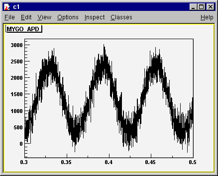
Examples :
Suppose a time series vector
vect
contains data starting at t=0, and has a duration of 1 s, with 50000
samples.
gVM->Draw(vect)
will draw the entire series.
gVM
->Draw(vect,0.3,0.2) will draw
the series starting at t0=0.3 s for a duration of 0.2 s, which
represents 10000 samples.
gVM
->Draw(vect,"same") will draw
the entire series on the same plot as a previous draw.
Drawing the distribution (histogram) of the
data contained in an FrVect
Makes a distribution of the values
contained in a series. This method generates or uses a histogram of the class
TH1F. If the histogram is generated, its limits are determined automatically to
be +/- 5% of the max and min value in the series and this histogram has 100
bins.
The variables are :
offset
is the offset from which the histogramming starts, with respect to the starting
value of the series.
dur
is the length of the histogramed part of the series.
hwork
is, optionally, the name of an existing histogram, for example "histo1". This
allows using any limits for the histogram, provided the user defines one before
calling DrawHist. The contents of the histogram are erased before filling by the
new values, except if a "+" precedes the name, as in "+histo1". In this case,
the data is appended to the histo. If the name hwork is given but there is no
already existing histogram of that name, a new one is created with standard
characteristics.
option
is an option string that is passed to the drawn histogram of type TH1F. This is
equivalent to the TH1 class drawing options. The reader can go to the address
http://root.cern.ch/ to see the list of options in the drawing of a TH1 (see
Classes and Members Reference Guide).
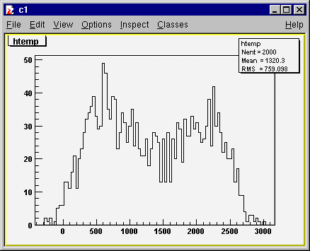
Examples :
Let's assume that a time series
vect
contains data starting at t=0, and has a duration of 1 s, with 50000 samples.
The min value is -123, the max value is 212.
gVM->DrawHist(vect,0.2,0.4)
will draw the histogram of the values in
vect beginning at t0=0.2 s for a duration of 0.4 s. The generated
histogram has limits [-130,223].
h1 = new TH1F("h1","test
histo",100,-25,25);
gVM->DrawHist(vect,0.2,0.4,"h1");
will generate the histogram
h1,
with limits [-25,25]. Calling the DrawHist method will fill this histogram but
only with the values in its range. So one can concentrate on the distribution of
values around 0.
gVM->DrawHist(vect,0.2,0.4,"+h1");
This will do the same thing as before but
without erasing the values of the histogram before filling. It will just add
those to the existing ones. That way, one can span more than one series for one
given histogram.
VII.2.4.2 Drawing
selected contents or distribution of a frame
One can draw a selected adc or processed or
simulated data without having to extract it first from a frame.
Simple drawing of a vector (1D or 2D)
contained in a frame :
frame
is a frame of type FrameH that has been read from a file.
typeAndName
is a pointer to an array of char
that describes the type (adc, proc or sim) and name of the frame element to be
extracted and drawn. It has the following structure : "type.name". For example
"adc.IFO_DMRO" is a good format. It will look for the adc data of the adc named
"IFO_DMRO". It is possible to give only the name, if there is no ambiguity. In
that case, adc data will be searched first for that name, then proc and then sim
data. If more than one identical name was used, the first found series will be
extracted.
offset
is the offset from which the drawing starts, with respect to the starting value
of the vector (i.e. series).
dur
is the length of the drawn part of the vector (i.e. series).
option
is an option string that is passed to the plot that is drawn. This is equivalent
to the TH1 class drawing options. The reader can go to the address
http://root.cern.ch/ to see the list of options in the drawing of a TH1 (see
Classes and Members Reference
Guide).
Options
:
The ones of the TH1 class, for example "same"
which superimposes a plot to a previous draw.
"sameti" does a similar superposition but
respects the time, i.e. will shift the plot so that it's time and the one of a
previously drawn vector
coincide.
If
offset
and
dur
are omitted, the whole vector is drawn. It is also possible to specify only the
drawing option.
A VSPlot is drawn in the current pad or
canvas. The address of this plot is added to the list of plots managed by this
manager. The name of the plot becomes the name of the FrXXXData extracted (XXX =
Adc, Proc or Sim).
Examples :
Suppose a FrAdcData vector
"MYGO_ADC"
contains data starting at t=0, and has a duration of 1 s, with 50000 samples in
a frame called
"frame".
gVM->Draw(frame,"adc.MYGO_ADC")
will draw the entire series.
gVM
->Draw(frame,"MYGO_ADC",0.3,0.2)
will draw the series starting at t0=0.3 s for a duration of 0.2 s,
which represents 10000 samples. Since no type (adc proc or sim) was given, it
will search for the first data occurring with this name in the
frame.
Example of such a plot :
gVM
->Draw(frame,"MYGO_ADC","same")
will draw the entire series on the same plot as a previous
draw.
Drawing the distribution (histogram) of the
data of a vector contained in a frame
Makes
a distribution of the values contained in a vector of type FrXXXData (XXX = Adc,
Proc or Sim) contained in the frame "frame" and of type and name
typeAndName.
This method generates or uses a histogram of the class TH1F. If the histogram is
generated, its limits are determined automatically to be +/- 5% of the max and
min value in the series and this histogram has 100 bins.
The variables are :
frame
is a frame of type FrameH that has been read from a file.
typeAndName
is a pointer to an array of char
that describes the type (adc, proc or sim) and name of the frame element to be
extracted and drawn. It has the following structure : "type.name". For example
"adc.IFO_DMRO" is a good format. It will look for the adc data of the adc named
"IFO_DMRO". It is possible to give only the name, if there is no ambiguity. In
that case, adc data will be searched first for that name, then proc and then sim
data. If more than one identical name was used, the first found series will be
extracted.
offset
is the offset from which the histogramming starts, with respect to the starting
value of the series.
dur
is the length of the histogramed part of the series.
hwork
is, optionally, the name of an existing histogram, for example "histo1". This
allows using any limits for the histogram, provided the user defines one before
calling DrawHist. The contents of the histogram are erased before filling by the
new values, except if a "+" precedes the name, as in "+histo1". In this case,
the data is appended to the histo. If the name hwork is given but there is no
already existing histogram of that name, a new one is created with standard
characteristics.
option
is an option string that is passed to the drawn histogram of type TH1F. For the
time being, this is equivalent to the TH1 class drawing options. The reader can
go to the address http://root.cern.ch/ to see the list of options in the drawing
of a TH1 (see Classes and Members Reference
Guide).
Examples :
Let's assume that a FrAdcData vector
contains data starting at t=0, and has a duration of 1 s, with 50000 samples.
The min value is -123, the max value is 212 in a frame called
"frame".
gVM->DrawHist(frame,"adc.MYGO_ADC",0.2,0.4)
will draw the histogram of the values in the
adc
"MYGO_ADC"
beginning at t0=0.2 s for a duration of 0.4 s. The generated
histogram has limits [-130,223].
Example of such a plot :
h1 = new TH1F("h1","test
histo",100,-25,25);
gVM->DrawHist(frame,"MYGO_ADC",0.2,0.4,"h1");
will generate the histogram
h1,
with limits [-25,25]. Calling the DrawHist method will fill this histogram but
only with the values in its range. So one can concentrate on the distribution of
values around 0. Since no type (adc proc or sim) was given, it will search for
the first data occurring with this name in the frame.
gVM->DrawHist(frame,"MYGO_ADC",0.2,0.4,"+h1");
This will do the same thing as before but
without erasing the values of the histogram before filling. It will just add
those to the existing ones. That way, one can span more than one series for one
given histogram.
VII.2.4.3 Drawing
2D vectors (images or time-frequency plots)
Frame vectors may contain bi-dimensional
information such as images coming from cameras or time-frequency plots. There is
no special method for drawing these 2D plots. One uses gVM->Draw() methods as
for 1D and these methods take care of producing the right plot, 1D or 2D
depending on the dimension of the data.
In the case of 2D, the plot produced is of
type VSPlot2. The manager handles a list of these plots, as well as a list of 1D
plots.
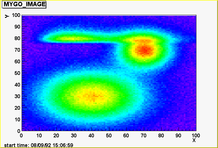
Example :
In the files produced by the create_testfr.C
script in the vegatutorial directory, some frames contain images. They are
generated as a sum of two dimensional functions and are there only for
demonstration purposes. Once in vegatutorial, the following lines should show an
image:
first, open a database
vega[]
vd = new VFrDataBase("demoDB.root")
second, extract the first frame of this
database
vega[]
fr = vd->GetNextFrame()
third, since the name of the vector
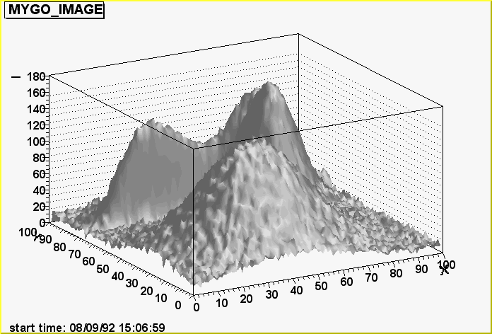
containing the image is "MYGO_IMAGE", plot it
vega[]
gVM->Draw(fr,"MYGO_IMAGE","col")
That's it ! The option "col" used for this
drawing produces the third plot showed hereafter, other options are
shown.
No option (scatter
plot)
Option
"surf1"
Option
"col"
Option
"surf4"
The options available are the ones of the
ROOT TH2 class and are summarized below:
Superimpose on previous picture in the same
pad
Use Cylindrical
coordinates
Use Polar coordinates
Use Spherical
coordinates
Use PseudoRapidity/Phi
coordinates
Draw a lego plot with hidden line
removal
Draw a lego plot with hidden surface
removal
Draw a lego plot using colors to show the
cell contents
Draw a surface plot with hidden line
removal
Draw a surface plot with hidden surface
removal
Draw a surface plot using colors to show the
cell contents
same as SURF with in addition a contour view
drawn on the top
Draw a surface using Gouraud
shading
Draw a contour plot (same as
CONT0)
Draw a contour plot using surface colors to
distinguish contours
Draw a contour plot using line styles to
distinguish contours
Draw a contour plot using the same line style
for all contours
Draw a contour plot using fill area
colors
Draw a contour plot using surface colors
(SURF option at theta = 0)
Generate a list of TGraph objects for each
contour
Arrow mode. Shows gradient between adjacent
cells
A box is drawn for each cell with surface
proportional to contents
A box is drawn for each cell, with a color
scale varying with contents
With LEGO or SURFACE, suppress the
Back-Box
With LEGO or SURFACE, suppress the
Front-Box
Draw plot, but not the axis labels and tick
marks (for LEGO and SURF options)
Draw a color scale on the right of the plot
(for COL and CONT options only)
Draw a scatter-plot
(default)
Since an image is attached to a given frame
and does not span two or more of them, one cannot, for the moment, extract a 2D
vector spanning two or more frames. One could indeed think of it for
time-frequency vectors but it is not yet done.
VII.2.5 Change
of the plots attributes
Once drawn, it is possible to change the
plots attributes like line color or fill style directly using gVM. The following
methods are available :
GetXaxis(const char*
name="")
GetYaxis(const char*
name="")
GetZaxis(const char*
name="")
Return a pointer to the specified axis
object, allowing to manipulate it.
The arguments are self explanatory, except
the name. This is the name of the plot on which the change of attribute should
be done. If name="", the change is applied to the last plot drawn by
gVM.
Examples:
gVM->SetMarkerSize(1.2)
will change the marker size of the last plot
drawn
gVM->SetLineColor(3,"MYGO_ADC1")
will change the line color of the plot named
"MYGO_ADC1".
VII.2.6 Management
of the plots produced
The manager decides at drawing time what is
the dimension of the plot produced depending on the dimension of the data in the
frame vector. If the frame vector is 1 dimensional, it produces a VSPlot, and if
it is 2D, it produces a VSPlot2. The manager then handles two lists of produced
plots, one for 1D and one for 2D.
One can get a pointer to the last created
and plotted VSPlot:
VSPlot*
GetLastPlot()
As
in :
vega[]
VSPlot* vs1 = gVM->GetLastPlot()
This could be useful if one wants to modify
this VSPlot, for example to change some attributes. An example is given in the
macro "peak2.C".
One can also get a pointer to the last
created and plotted VSPlot2 :
VSPlot*
GetLastPlot2()
As
in :
vega[]
VSPlot2* vs1 = gVM->GetLastPlot2()
This could be useful if one wants to modify
this VSPlot2, for example to change some attributes.
VII.3 Representing
slow monitoring data
There are three main powerful drawing
methods for slow monitoring data, i.e. VNtuples. They all enable putting
selections, i.e. drawing data that pass given cuts.
The first method draws VSPlots, which are
standard representations of time series. This method is mainly used to treat
slow monitoring data as simple time series. We encourage you to use this first
method since it gives powerful manipulation (signal analysis)
capabilities.
varlist
is an expression of the general form e1:e2 where e1,etc is a formula referencing
a combination of the ntuple columns
Example: varexp = x:y simplest
case: draw a plot of points (x,y), x and y representing columns named x and
y = t:sqrt(x) :
draw plot of sqrt(x) vs t =
log(t):x*y/z Note that the variables
e1 or e2 may contain a selection.
example, if e1= x*(y<0), the value plotted will be x if y<0 and will be 0
otherwise.
cuts
is a selection expression. Only ntuple entries passing this selection will enter
into the graph. For example, it could be something like “t>10
&& sin(TP1/6.28) <0”. One can use standard C operators (+ - * /
&& || !...) and usual mathematical functions, including transcendental
ones.
option
is an option for drawing. The available options are
:
option = 'A'
Axis are drawn around the
graph
option = 'T'
Time is used for axis labels (not a standard
graph feature, added by VEGA)
option = 'P'
The current marker is drawn at each
point
option = 'L'
A simple polyline between all the points is
drawn
option = 'F'
A fill area is drawn ('CF' draw a smooth
fill area)
option = 'C'
A smooth Curve is
drawn
option = '*'
A Star is plotted at each
point
option = 'B'
A Bar chart is drawn at each
point
Options should be combined to obtain the
desired effect. Typically, the first graph is drawn with option 'AP', to draw
the axis, and subsequent plots that the user wants to overlay are plotted with
the 'P' option alone.
nentries
is the maximum number of entries to be processed in the ntuple
firstentry
is the first entry to be processed
The second method draws histograms. This is
mainly used for statistical studies.
Unlike in DrawGraph, which needs at least
two variables to plot a graph, one can plot a 1D, 2D or 3D histogram. The
variables have the same meaning as in DrawGraph() but the varlist can contain
the name of an existing histo and options are not the same :
varlist
is an expression of the general form e1:e2 where e1,etc is a formula referencing
a combination of the ntuple columns
Example: varexp = x:y simplest
case: draw a plot of points (x,y), x and y representing columns named x and
y = t:sqrt(x) :
draw plot of sqrt(x) vs t =
log(t):x*y/z Note that the variables
e1 or e2 may contain a selection.
example, if e1= x*(y<0), the value plotted will be x if y<0 and will be 0
otherwise. One can save the result of
Draw to a histogram:
===================================
By default the temporary histogram created is called
htemp. If varlist contains
>>hnew (following the variable(s) name(s), the new histogram created is
called hnew and it is kept in the current directory (See the class TDirectory of
ROOT).
Example: vnt->Draw("sqrt(x)>>hsqrt","y>0")
will draw sqrt(x) and save the histogram as "hsqrt" in the current
directory.
By default, the
specified histogram is reset. To continue to append data to an existing
histogram, use "+" in front of the histogram
name; vnt->Draw("sqrt(x)>>+hsqrt","y>0") will
not reset hsqrt, but will continue filling.
option
is an option for drawing The following
options are supported on all
types:
"SAME"
Superimpose on previous picture in the same
pad
"CYL"
Use Cylindrical
coordinates
"POL"
Use Polar coordinates
"SPH"
Use Spherical
coordinates
"PSR"
Use PseudoRapidity/Phi
coordinates
"LEGO"
Draw a lego plot with hidden line
removal
"LEGO1"
Draw a lego plot with hidden surface
removal
"LEGO2"
Draw a lego plot using colors to show the
cell contents
"SURF"
Draw a surface plot with hidden line
removal
"SURF1"
Draw a surface plot with hidden surface
removal
"SURF2"
Draw a surface plot using colors to show the
cell contents
"SURF3"
same as SURF with in addition a contour view
drawn on the top
"SURF4"
Draw a surface using Gouraud
shading
The following options are supported for
1-D
types:
"AH"
Draw histogram, but not the axis labels and
tick marks
"B"
Bar chart option
"C"
Draw a smooth Curve through the histogram
bins
"E"
Draw error bars
"E0"
Draw error bars including bins with o
contents
"E1"
Draw error bars with perpendicular lines at
the edges
"E2"
Draw error bars with
rectangles
"E3"
Draw a fill area through the end points of
the vertical error bars
"E4"
Draw a smoothed filled area through the end
points of the error bars
"L"
Draw a line through the bin
contents
"P"
Draw current marker at each
bin
"*H"
Draw histogram with a * at each
bin
The following options are supported for
2-D types:
"ARR"
arrow mode. Shows gradient between adjacent
cells
"BOX"
a box is drawn for each cell with surface
proportional to contents
"COL"
a box is drawn for each cell with a color
scale varying with contents
"COLZ"
same as "COL". In addition the color mapping
is also drawn
"CONT"
Draw a contour plot (same as
CONT3)
"CONT0"
Draw a contour plot using colors to
distinguish contours
"CONT1"
Draw a contour plot using line styles to
distinguish contours
"CONT2"
Draw a contour plot using the same line style
for all contours