II An
interactive session
In this first chapter, we will concentrate on giving the reader a feeling
of the possibilities of the framework. We will use standard ROOT as well as VEGA
specific examples.
The user actions will be written in bold characters.
II.1 Basic
intrinsic operations
First of all, one needs to know how to exit from a program! The C
interpreter has some raw commands that begin with a dot. These commands are used
to do intrinsic operations, not related to any C/C++ code. The ones that you
should know for the beginning are:
|
.q
|
quits the interactive session
|
|
.x
|
loads a macro and executes it
|
We will see other raw commands, as we need them, especially commands to
debug scripts (step, step over, set breakpoint, etc...).
II.2 The
interpreter CINT, graphical interaction through a few examples
II.2.1 First
very simple example
First, go to the $ROOTSYS/tutorials and start the ROOT/VEGA interactive
session:
your_prompt$ vega
The prompt that you see is "vega[]". In fact, you launched the
very small vega executable, which is in $VEGA/$UNAME and which is linked with
the ROOT libraries.
This program gives access via a command-line prompt to all available
ROOT/VEGA classes/globals/functions. By typing C/C++ statements at the prompt,
you can create objects, call functions, execute scripts, etc. For example
type:
vega[] 1+sqrt(9)
(double)4.000000000000e+00
vega[] for (int i = 0; i<5; i++) printf("Hello %d\n",
i)
Hello 0
Hello 1
Hello 2
Hello 3
Hello 4
vega[] .q
As you can see, if you know C or C++, you can use ROOT. No new command line
or scripting language to learn.
Some comments may be made at this point. First, there is no need to put a
semicolon at the end of a line. Well, you can put one if you want. This is only
true for statements written on the command line. One assumes that the carriage
return is enough to express the end of the line for the interpreter. This is
part of the interpreter’s extensions to C++ that were made to allow an
easy interaction, while not at the expense of breaking the compatibility with
C/C++ language.
Some of the extensions don’t work anymore inside a macro. For
example, you have to put a semicolon at the end of each line in a
macro.
II.2.2 Graphical
output example
Let’s try something more interesting. Again, start VEGA :
your_prompt$ vega
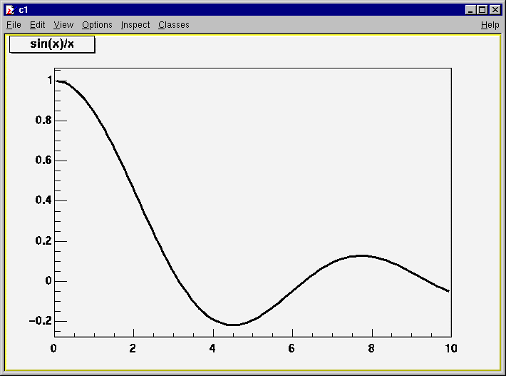
vega[] TF1 f1("func1", "sin(x)/x", 0, 10)
vega[] f1.Draw()
you should see something like this :
II.2.3 Classes,
methods and constructors
In ROOT and C++, we introduce the notion of object, which is just a C
structure with some internal functions (called “methods”) associated
to it.
The line TF1 f1("func1", "sin(x)/x", 0, 10) created an
object named f1 of the type TF1 which is a
one-dimensional function. The type of an object is also called a
class.
In fact, the line above builds an object by giving it a set of parameters.
This is one example of a function associated to a class. It is a special one
since it builds an object. It is called a constructor.
To interact with an object in ROOT, the usual syntax is :
object.action(parameters)
This is the usual way of doing in C++. The dot can be replaced by -> if
object is a pointer. But since the interpreter always knows the type (class) of
an object, if you put a dot instead, it will be automatically replaced when
necessary.
So now, we understand the two lines that allowed us to draw our function.
f1.Draw() means “call the method Draw associated with the
object f1 of class TF1”. We will see the advantages of using objects and
classes very soon.
One point : the ROOT framework was designed as an object oriented
framework. This doesn’t mean that a user cannot call plain functions. For
example all the FrameLib standard functions are available in the VEGA
framework.
II.2.4 ROOT
related specifics
We didn’t yet explain everything about the constructor of f1
:
TF1 f1("func1", "sin(x)/x", 0, 10)
"sin(x)/x" is the function that we want to define, 0 and 10 the
limits but what is "func1”? It’s the name that we give to
the object f1. Most objects in ROOT have a name. That way, there are lists of
objects maintained by ROOT and it’s easy to find an object by its name,
especially if it is in a database. We will see why it is so when we see the
notion of inheritance.
II.2.5 Graphical
output example: User interaction
If you quit the framework, try to draw again the function
"sin(x)/x". Now, we can look at some interactive capabilities. Every
graphics drawn in a window (which is called a Canvas) is in fact a graphical
object in the sense that you can grab it, resize it, change some characteristics
with a mouse click. And all the changes that you do are not done on a graphical
copy of the object but on the object itself. For example try to click somewhere
on the x-axis and drag along this axis. You have a very simple zoom.
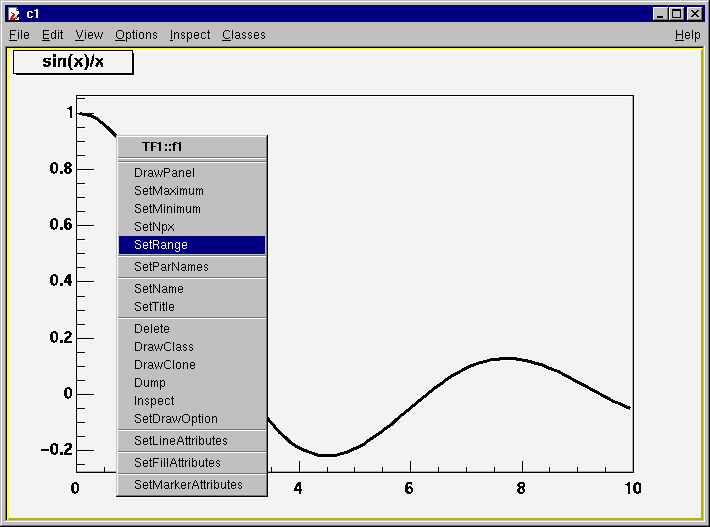
When the cursor is on any object, you have access to selected methods by
pressing the right mouse button and obtaining a context menu showing some
available methods for this object. If you try this on the function itself, you
obtain this kind of behavior:
You can try for example to select the SetRange method and
put -10, 10 in the dialog box fields. This is equivalent to executing the member
function f1.SetRange(-10,10) from the command line prompt,
followed by f1.Draw().
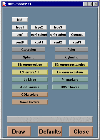
There are other things you may want to try. For example select the
"DrawPanel" item of the popup menu. You will see a panel like this one
:
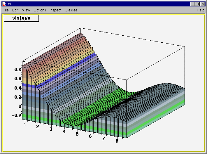
Try to resize the bottom slider and click Draw. You can zoom your graph. If
you click on "lego2" and "Draw", you see a 2D representation of your graph
:
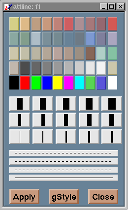
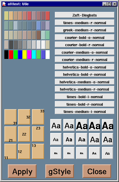
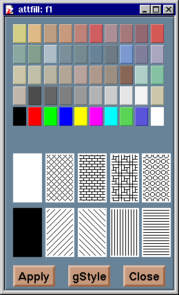
You can rotate interactively this 2D plot. Of course, it is possible to
plot real 2D functions or graphs, not only a disguised 1D. There are numerous
ways to change the graphical options/colors/fonts with the various methods
available in the popup. Here are a few examples:
|
|
|
|
Line attributes
|
Text attributes
|
Fill attributes
|
Once the picture suits your wishes, you may want to see what are the lines
of code you should put in a macro to obtain the same result. To do that, choose
the "Save as canvas.C" option in the "Files" menu. This will generate a macro
that you can look into to see how to set the various options. Notice that you
can also save in postscript or gif formats the picture.
One other interesting possibility is to save in native root format your
canvas. This will enable you to open it again and to change whatever you like,
since all the objects associated to the canvas (histograms, graphs, etc...) are
saved at the same time.
II.2.6 Second
example : Building a multi-pad canvas
Let’s now try to build a canvas (i.e. a window) with several Pads.
The pads are sub-windows that can contain other Pads or graphical
objects.
vega[] can = new TCanvas("can","Test canvas",1)
vega[] can.Divide(2,2)
Once again, we called the constructor of a class, this time the class
TCanvas. The difference with the previous constructor call is that we want to
build an object with a pointer to it. In C, we would have used malloc() or
calloc(). Here, we use the operator new, which is the equivalent in C++.
Instead of free() we will use delete. Usually, one has to declare a
variable before using it. Since there cannot be any ambiguity in the line above,
one doesn’t need to declare a variable “can”. In case such a
statement in a macro is intended to be compiled, one would obviously have to
declare the variable as a TCanvas* before using it.
Next, we call the method Divide() of the TCanvas class (that is
TCanvcas::Divide()) which divides the canvas into 4 zones and sets up a Pad in
each of them. Now, if we do
vega[] can.cd(1)
vega[] f1.Draw()
the function f1 will be drawn in the first Pad. All subsequent actions,
draw an arrow for example, will be done on that Pad. To change the working Pad,
there are three ways:
- Click on the middle button of the mouse on an object, for example a Pad.
This sets this pad as the active one
- Use the method cd() of TCanvas (that is TCanvas::cd()) by telling the number
of the pad, as was done in the example above:
vega[]
can.cd(3)
Pads are numbered from left to right and from top to bottom.
- Each new pad created by the TCanvas::Divide method has a name, which is the
name of the canvas followed by _1, _2, etc... for example to cd() to the third
pad, you should do :
vega[] can_3.cd()
The third pad will set itself as the selected pad since you call the
TPad::cd() method for the object can_3. This remark just to show the state of
mind people have when they "think" in C++
II.2.7 Inheritance
and data encapsulation
II.2.7.1 Inheritance
There is an obvious question that could be asked : what is the relation
between a canvas and a pad ? Isn’t it almost the same thing? Yes it is. In
fact, a canvas is a pad that spans through an entire window. This is
nothing else than the notion of inheritance. The TPad class is the parent of the
TCanvas class.
So what? The most interesting thing is that you can reuse the code written
in the parent class. For example, cd() is a method that TCanvas inherits from
it’s parent, TPad.
II.2.7.2 Method
overriding
The method overriding is explained in chapter IV. Basically, when a class
Child derives from another class Parent, it can reuse the methods defined in
Parent, but if one method of Parent is not well adapted to Child, one can
redefine (override) it. For example Draw() in some Child class may be different
from Draw() in the Parent class. There is no ambiguity since you always specify
the object : childobject.Draw() or parentobject.Draw().
II.2.8 ROOT
related specifics
For what concerns inheritance, most objects in ROOT derive from a base
class called TObject. This class contains everything that is shared by all the
classes in ROOT. Especially, it handles
- the object I/O, so one can send any object to a file without writing the
corresponding code,
- comparing two objects, enabling searches, sorts, etc...
- graphics hit detection
- notification between objects, so they can talk to each
other...
to name the most important ones.
II.3 An
example of a macro
Let's try now to see how we can write a simple macro. As we've said, this
is just C/C++ code. Open the editor of your choice and look at the macro named
vfill_histo.C. As a matter of convention, all macros are suffixed by .C. The
source code has a .cxx or .cc suffix. vfill_histo.C is the following code
:
- {
- // Create and fill a histogram with random #'s from a Gaussian
distribution.
- // See http://root.cern.ch/root/HowtoHistogram.html for a brief
description
- // of how to use histograms in ROOT.
- gROOT->Reset();
-
- // TH1F is the equivalent of HBOOK1
- // The fill data are 32 bit float points and weights are 64 bit
fp.
- printf("Creating Histogram...\n");
- TH1F *h1 = new TH1F("h1","1-D Gaussians",100,-8,8);
- printf("done.\n");
-
- //The ROOT/CINT extensions to C++. The declaration of h1 may
be
- //omitted when "new" is used. So h1 = new TH1F(...) will correctly
- //create an object of class "TH1F".
- gRandom->SetSeed();
-
- // Raw C types are typedefed.
- Float_t xgauss;
- printf("Filling Histogram...\n");
- for (Int_t i=0; i < 10000; i++) {
- xgauss = gRandom->Gaus(3,0.5);
- h1->Fill(xgauss,0.2);
- h1->Fill(xgauss-6);
- }
- printf(" done.\n");
- }
We can try to give detailed explanations of some of the lines
above.
- gROOT->Reset();
This statement resets the interpreter environment, it is almost always used
at the beginning of a macro but not if you want to preserve some variables that
a precedent macro defined. gROOT is a global variable. We will see some more
details about globals in ROOT in a few moments. gROOT is an object of the class
TROOT, which represents your session. It contains, among other things, lists of
named objects created during the session, such as histograms. This enables
access to those objects by their name.
- TH1F *h1 = new TH1F("h1","1-D
Gaussians",100,-8,8);
Here, we create a histogram by invoking one of its constructors. Walking
through this statement, we have :
- TH1F: this is one of the histogram classes. All ROOT classes begin with a T
(see Coding Conventions). As we will see, all VEGA classes begin with a V. H is
for histogram, 1 for 1-D and F for using one float per channel.
- *h1 is the name of the pointer to this object
- new TH1F(...) invokes the constructor for this object with several
parameters:
- "h1" is the name of the histogram. In ROOT, as we have seen, most high level
objects are named. Typically, one makes the name of the object the same as the
pointer to which it refers.
- "1-D Gaussians" is the title of the histogram. It will be displayed by
default when the histogram is drawn.
- 100, -8, 8 are the number of bins nbins, xlow and xup. For PAW users : you
don't have to worry about the type of xlow and xup, integers will be converted
to floats.
- gRandom->SetSeed();
Another global. gRandom is the current object of the class TRandom of
standard random generators. You probably already noticed that all globals begin
with a "g" followed by a capital letter. This is general and belongs to the
coding conventions used in ROOT, which are followed by VEGA . The SetSeed()
method of TRandom chooses a random seed, here the default one.
The class TRandom doesn't try to be overly ambitious. The important methods
are :
- SetSeed(iseed) : sets the seed of the random number generator. If no number
is given, 65536 is used.
- Gaus(mean, sigma) : return a random number distributed following a gaussian
with mean and sigma.
- Rannor(a,b) : returns two random numbers following a gaussian with mean=0
and sigma=1.
- Rndm() : returns a uniformly distributed random number in the interval
[0,1]
- Float_t xgauss;
To avoid machine dependence of raw C types (double, float, and especially
int, etc...), the basic types have been typedefed. So, instead of float, we use
Float_t = 4 byte float. You can equally well use standard types (float, double)
for your everyday work. In VEGA, we integrated the Framelib, which has its own
machine-independent data types. To avoid problems, we decided to keep both. So
you can use Float_t (ROOT type) or REAL_4 (Framelib type) indifferently. We know
this can be misleading but one cannot avoid some historical
background...
- for (Int_t i=0; i < 10000; i++) {
- xgauss = gRandom->Gaus(3,0.5);
- h1->Fill(xgauss,0.2);
- h1->Fill(xgauss-6);
- }
This seems to be a standard for loop in C in which you generate a random
variable (gaussian) and you fill a histogram with this value.
For somebody not used to C++ something is strange : the Fill() method used
to fill the histogram is used twice but not with the same number of arguments.
This is perfectly common in C++, and it is called method overloading. We
will see more about this in the next paragraph.
Now, to execute your macro type :
vega[] .x vfill_histo.C
Creating Histogram...
done
Filling Histogram...
done
Now you have in your memory (the computer one, not yours...) a histogram
with which you can play. For example type
vega[] h1->Draw()
vega[] h1->Dump()
As will be seen in the chapter "Writing macros", one can write a named
macro and give arguments to a macro. You also probably noticed that there is no
includes in the macro. In fact, all the standard C includes are already done in
the environment, as well as ROOT and VEGA specific ones.
II.3.1 C++
notions used: method overloading
We've just seen, in the example above, that a method can have different
forms, with different arguments. If we look at an excerpt of the header file
defining the class TH1F :
- public:
- virtual void Fill(Axis_t x);
- virtual void Fill(Axis_t x, Stat_t w);
- virtual void Fill(Axis_t x, Axis_t y, Stat_t w);
- virtual void Fill(Axis_t x, Axis_t y, Axis_t z, Stat_t
w);
You see that the Fill method is defined four times with different arguments. How does the compiler know what method to call ?
For the compiler to be able to make the difference, the arguments must be
different enough. There is no ambiguity in the Fill methods above since the
number of parameters is different for each method. If someone had made the
following statement :
- public:
- virtual void Fill(Axis_t x);
- virtual void Fill(Axis_t x, Stat_t
w=1);
where in the second declaration, one of the arguments has a default value
(this is permitted in C++), then the compiler doesn't know which method to call
if someone uses
- h1->Fill(23)
Should the compiler use the form Fill(Axis_t x); where x=23 or the
form Fill(Axis_t x, Stat_t w=1); where x=23 and one uses the default
value w=1 ?
In that case, the compiler sends an error message. So one must be careful,
when writing his methods not to come in such situations. Easier said than
done.
II.4 How
to compile a macro ?
Sometimes (in fact quite often) a script may become so big or be so
processing-hungry that one would like to have it compiled and not interpreted.
There is included into ROOT what is called a script compiler that allows
compiling very easily the scripts you are going to produce.
It starts by calling the C++ compiler that was used to build ROOT and
builds a shared library. This shared library is then loaded and the function
defined in the script is executed.
II.4.1 Preparation
of the script
So that seems nice, what is the deal ? It’s only that you have to
prepare a little bit your script. But it is quite simple. You have to
- NOT use extensions to C/C++ provided by the CINT interpreter. That means for
example that while in the interpreter you do not need to declare variables whose
type is known from the context, this is mandatory if you want to be able to
compile. Since the compiler is not supposed to know the context of the
interpreter. An example. In the interpreter, you can use statements like
:
c1 = new TCanvas("c1", "Test",1);
where you do not
declare the variable c1, you should do instead :
TCanvas*
c1 = new TCanvas("c1", "Test",1);
More generally, use very standard
C/C++ and declare all your variables
- You should add includes you use at the beginning of the file. Once again,
this is for the real compiler that will do the work. Usually, the headers to be
added are composed of the name of the classes used followed by the .h suffix. In
case of included C code, the most commonly used are "FrameL.h" for all
the Framelib calls, and the standard headers of the Virgo standard signal
library.
- In case you want to execute immediately (i.e. use the command
“.x”) the first function of the script you compile, you have to name
the function in your script with the same name as the file it is contained in.
For example the file my_test.C should begin with
my_test()
{
your code....
}
The tutorial script called scrollspectrum.C has been prepared this
way, check it.
II.4.2 Compiling
the script
What remains to be done is to compile the script. If we want to execute the
script called scrollspectrum.C, we just have to do (once in the
vegatutorial directory) :
vega[] .x scrollspectrum.C++
notice the ++ at the end of the command. This tells the interpreter to
compile scrollspectrum.C, build a shared library called
scrollspectrum.so, load this shared lib and execute
scrollspectrum().
The resulting library scrollspectrum.so stays here and you can reuse it,
that is reload it at a later time, with
vega[] .L scrollspectrum.so
furthermore, the scrollspectrum() function is available in the interpreter
and may be used in some other script !
All this also works with loading the script after compiling :
vega[] .L scrollspectrum.C++
is a valid statement. This will build the library and load it as before. It
will just not execute any function.
II.4.3 Compiling
a more complex code
You will probably at one point or another try to compile a more complex
code, consisting of a few files, or you will want to use the VEGA capabilities
in your own code, for example use the display of vectors in a standalone
executable. This is described in the chapter “How to compile your own code
for VEGA or use the VEGA libraries in your code” at the end of the
manual.
Damir BUSKULIC
Last update :19/11/2001;