Before describing extensively the VEGA classes, methods and objects, it would be interesting to put directly hands on the environment and see some of it's capabilities from the point of view of gravitational waves data analysis. Concepts will be introduced as needed.

So, let's imagine someone has a set of frame files that he/she wants to analyze. We will first build some tutorial files. Copy to your home directory the "vegatutorial" directory that is in the VEGA package. Then cd to this directory and launch a VEGA session. Then, in this session, execute the create_testfr.C script :

This will create files containing a few test frames, starting at time (GPS) 400000000.097, till the time 400001475.097. You will see some plots of the contents of these frames at the same time. Then, a file named SMSdemo.F containing frames with only slow monitoring test data will be produced.

Now that we have a few frame files, we will need to access quickly a subset of them, if possible without bothering with frame boundaries, just giving the start time and length of the piece we want. Indeed, it is possible and the mechanism that allows such a thing in VEGA is the metadatabase. This database indexes all the files and the frames they contain and is able to extract a vector of any length, starting at any time.

Let's build such a database with the demo frame files :

The operator new, described elsewhere, is creating an object of the class VFrDataBase, returning a pointer v . The arguments of the constructor are first the name of the ROOT file that will hold the database (in our case "demoDB.root"), next the mode of opening ("READ" by default, but we used "CREATE" to build a new database). The third argument is the path to the files. As can be seen, one can use wildcards to specify frame files names. But one could as well specify a directory name. The search is by default recursive, which means you can set the beginning of the search to the top of a directory tree containing directories, etc....

Now, we can try to open an existing database :

NOTE : Since it's annoying to always type long names, one can use the tab completion feature of ROOT, using the <Tab> key :

and the name is completed automatically. This is also true for names of files in the current directory. Even more, if you write :

You will have the list of variables used by this method, with the default parameters, and all the possible versions. This is VERY helpful.

Now, as advertised, you can extract a frame from the set of files with :

To see the contents of the frame, one can do the standard Framelib call :

Which gives a summary of the contents of the frame. One can see that there is an ADC channel named MYGO_ADC1. But you can have the same kind of information from the database itself by issuing

This will print all kinds of information about the database and dump the contents of the first frame.

To draw the previously extracted frame in the current pad, just do :

Woaw ! what is this new beast, "gVM" ?

Well, if we wanted to be consistent with the "Object Oriented" way used in ROOT, we would have needed to use a fully C++ version of the Framelib. But this would have meant a complete change of the habits of many people. Since people are used to the C version, and since at the moment, the C++ version is not quite ready, we preferred to use a "manager class" that is taking the Framelib objects and building graphical objects with them. This class is called VManagerFrameL.

At initialization time, a global variable of type VManagerFrameL is build, called gVM and it is available for all kinds of management tasks, taking care of drawn plots, freeing memory when necessary, taking care of a reference time, etc...

So, the last command we did created a plot (graphical representation, class VSPlot) of the frame fr content, more specifically of the adc channel named "MYGO_ADC1". The "adc" characters may be omitted if there is only one vector (adc proc or sim) with that name.

Even if it is supposed to be only a graphical representation of a vector, a VSPlot is much more than that. In fact, it contains almost all the information contained in a time series (FrVect for example). It can be the starting object for a truly "OO" way of doing time series.

For the moment, let's access the VSPlot object that was created :

It was said that the VManager called gVM takes care of all the drawn plots. This instructs gVM to return us a pointer to the last drawn plot.

Now we can do things like

You can always use <Tab> to see the available methods. Furthermore, one can click on the drawn line or plot with the third mouse button, have a popup menu and select methods like we did for histograms. The interactive zoom is also available.

It is also possible to plot images coming from cameras that are included in a frame as FrVects in 2 dimensions. One uses the same syntax as for 1D, the manager gVM will take care of producing the right plot.

The tutorials contain a few examples of the use of gVM (see the macros scroll2.C and peak2.C for example).

What if I don't want to take care of frame boundaries, I just want to see a vector containing MYGO_ADC1 data, beginning at the time 400000023 and lasting 10 seconds ?

The database can give you that. Do :

The first line extracts the vector, the second draws it. Notice that you didn't care about the frame boundaries, one of which is around 400000024.5, the other around 400000030.

Of course, one can extract a vector as big (or as small) as he wants, limited by the available machine memory of course.

One note : the user should take care of freeing the memory for all Framelib objects that are returned. Once a FrVect or a FrameH is extracted, it is the user's responsibility to free memory in his loops with FrameFree(fr) and FrVectFree(ve). In a future version, we will try to do an automatic garbage collection, to free (!) the user from these tasks. For the moment, this is not so important since the amount of created vectors/frames is not big.

The vectors inside a frame may be two dimensional and may represent an image coming from a camera. 2D vectors are plotted the same way as 1D vectors. For example, assuming ve2 is a 2D vector (of type FrVect):

will draw it.

Let’s see a concrete example, using the files contained or generated in the vegatutorial directory. First, open a database

second, extract the first frame of this database

third, since the name of the vector containing the image is "MYGO_IMAGE", plot it

That's it ! The option "col" used for this drawing produces a color plot. Other options are shown in the chapter “Representing gravitational waves data”

A few tutorials explain how to do it more generally: “moveimage.C”, “tifrdisplay.C” for example.

Frames are generally build with a certain set of conditions or selection parameters, coming from the online triggers or decided by the user. A user may want to process only a subset of the frames pointed to by a metadatabase, corresponding to some conditions, say amplitude of the trigger “Trig1” higher than a certain value.

When building the metadatabase, the trigger information is read from the frame and saved. This allows, when using it, to quickly browse the metadatabase searching for frames that obey a given set of conditions.

Let’s illustrate the use of this feature with our tutorial test files. We will suppose that w is the metadatabase pointing to these files, as opened in the previous paragraph. The frames contained in the tutorial files were generated with two trigger structures Trig1 and Trig2, which have various amplitudes for the various frames.

First, we may try to see the value of a given trigger amplitude by plotting it. The database object w (of type VFrDataBase*) has the capability to draw it:

This will plot the amplitude of the trigger Trig1 provided it is defined. The second string "Trig1" is a selection expression, so one can plot only the amplitude of selected triggers.

The second step is to define the selection expression, with a set of conditions, which will govern the search for specific frames. This is done by defining a new object, called a condition set (class VConditionSet), that will contain the selection expression and serve as a pointer to a specified position in the metadatabase:

The selection expression may use standard C operators and the main C math functions. "sin(Trig1.amp)>0.23 || Trig2==0" is a valid expression.

Now, one calls repeatedly the GetNextFrame(cs) method of VFrDataBase to get all the frames corresponding to the selection. To illustrate this, let’s load the next selected frame and see it’s beginning time :

Do not forget that fr is a FrameH structure and as such, we can use its internal variables, such as GTimeS, the start time.

You see that the start time is obviously far from the start time of the first frame (400000001). All the frames in between were skipped since they did not obey the selection expression.

If you use repeatedly GetNextFrame, do not forget to delete the object fr after it’s use (with FrameFree(fr)), otherwise your memory will get filled by all the undeleted frames that were passed to you.

Slow monitoring data spans a lot of frames. Thus, it requires a special treatment. To illustrate this, let’s build a database with frame files containing only SMS data. One such file was build by the create_testfr macro. Its name is SMSdemo.F. Check that you have such a file. Then, create a database with for example:

If you want to see the contents of the frames, do as before :

You will see that there is a slow monitoring station called MYGOSMS that contains two variables VF1 and VI2.

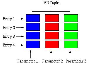
The special treatment we have to apply in order to gain a simple yet efficient way of dealing with SMS data is to build a special object called an ntuple that will contain all this data. We developed a particular ntuple that differs from the standard ROOT one in that it is adapted to our needs. You can think of a ntuple as a list of all the sms data put in a tree-like structure :

The difference with a simple array is that each leaf of the tree can be any kind of object, even a tree itself. This leads to a hierarchy structure, like in a directory structure for a file system.

In fact, these more general ntuples are called trees and we will not yet work with them. In simple ntuples, each leaf is a single float parameter.

So to build a ntuple starting from the slow monitoring data, one can do :

The first parameter "nt" is the name of the ntuple. Then, "MYGOSMS.VF1:MYGOSMS.VF2" is the list of SMS variables one wants to extract. Instead of telling every variable, you can specify only the name of a slow monitoring station, MYGOSMS in our case. The last two parameters are the start time from which we want the extraction and the length, expressed in seconds.

This ntuple will have three variables, the time being the first variable automatically inserted during extraction. If you want to see the contents of the ntuple, do :

Now that we have a ntuple, one can easily plot all sort of things. For example, if you want to plot the variations of VF1 with time :

The second, empty parameter is a selection parameter. One can overlay a second plot :

One can also use some complicated expressions, for example

Where you can see that the expressions can use the standard operators and simple mathematical functions.

One can also plot a histogram of some columns of the ntuple :

See the result and try to rotate interactively the drawn histogram.